Problem 1 a.
function [q, nfun] = adsimpson(f, a, b, tol)
    persistent recursion_depth nfun_internal;
    if isempty(recursion_depth)
        recursion_depth = 0;
    end
    if isempty(nfun_internal)
        nfun_internal = 0;
    end
    recursion_depth = recursion_depth + 1;
    nfun_internal = nfun_internal + 1; % Increment function evaluations

    if recursion_depth > 1000 % Check recursion depth
        error('Maximum recursion depth exceeded.');
    end

    c = (a + b)/2;
    h = b - a;
    fa = f(a); fb = f(b); fc = f(c);
    S = (h/6) * (fa + 4*fc + fb);

    d = (a + c)/2; e = (c + b)/2;
    fd = f(d); fe = f(e);
    Sleft = (h/12) * (fa + 4*fd + fc);
    Sright = (h/12) * (fc + 4*fe + fb);
    S2 = Sleft + Sright;

    if abs(S2 - S) < 15*tol
        q = S2 + (S2 - S)/15;
    else
        mid = (a + b)/2;
        [q_left, nfun_left] = adsimpson(f, a, mid, tol/2);
        [q_right, nfun_right] = adsimpson(f, mid, b, tol/2);
        q = q_left + q_right;
        nfun_internal = nfun_internal + nfun_left + nfun_right;
    end

    if nargout > 1
        nfun = nfun_internal;
    end

    recursion_depth = recursion_depth - 1;
    if recursion_depth == 0
        nfun_internal = 0; % Reset on the last exit
    end
end
b.
function q = dsimpson(f, a, b, c, d, tol)
    function qx = integrand_x(y)
        [qx, ~] = adsimpson(@(x) f(x, y), a, b, tol);
    end
    [q, ~] = adsimpson(@(y) integrand_x(y), c, d, tol);
end
The output are as follow
dsimpson 2.9491801536006179e-01
integral2 2.9491801499984915e-01
|dsimpson-integral2| =3.60e-10
Problem 2
function pendulum
    % Define the range for x values
    x_values = linspace(-0.99, 0.99, 200); % Adjust the number of points for smoothness
    K_values = zeros(size(x_values));
    evals = zeros(size(x_values));
    tol = 1e-10;

    % Define the integrand for the elliptic integral of the first kind
    for i = 1:length(x_values)
        x = x_values(i);
        integrand = @(theta) 1 ./ sqrt(1 - x^2 .* sin(theta).^2);

        % Use adsimpson to integrate and capture the number of function evaluations
        [K_values(i), evals(i)] = adsimpson(integrand, 0, pi/2, tol);
    end

    % Plot K(x) versus x
    figure;
    plot(x_values, K_values);
    title('Complete Elliptic Integral of the First Kind K(x) versus x');
    xlabel('x');
    ylabel('K(x)');

    % Plot the number of function evaluations versus x
    figure;
    plot(x_values, evals);
    title('Number of Function Evaluations versus x');
    xlabel('x');
    ylabel('Number of Function Evaluations');
end
The following graph are then produced

 Explanation
The graph show extreme spike at both end of the range, close to +-1
The graph shows an extreme spike in the number of function evaluations at both ends of the range, close to . This is consistent with the expectation that as approaches , the integrand of the complete elliptic integral of the first kind, , approaches a singularity for some within the interval .
When is near , the term can approach , causing the denominator to approach zero and the integrand to become very large or approach infinity, especially as approaches .
The adaptive Simpson’s method tries to maintain the specified tolerance by increasing the number of intervals (thus function evaluations) where the integrand varies rapidly or becomes difficult to approximate due to singular behavior. Near these singularities, even small intervals can have large differences in the integrand values, leading the adaptive algorithm to recursively subdivide the intervals, resulting in a substantial increase in function evaluations.
The sharp increase in function evaluations at the edges of the graph indicates that the algorithm is working as expected, refining the integration intervals to handle the challenging behavior of the integrand near the points where it is not well-behaved. The function evaluations become extremely high as the integrand requires very fine subdivisions to approximate the integral within the specified tolerance near the singular points.
Problem 3
C Trapezoidal rule
function I = trapezoid(f, a, b, n)
	% Composite Trapezoidal Rule
	x = linspace(a, b, n+1); % Generate n+1 points from a to b
	y = f(x);
	dx = (b - a)/n;
	I = (dx/2) * (y(1) + 2*sum(y(2:end-1)) + y(end));
end
C Simpson’s rule
function I = simpson(f, a, b, n)
	% Composite Simpson's Rule
	% Ensure n is even
	if mod(n, 2) == 1
		warning('Simpson’s rule requires an even number of intervals.');
		n = n + 1;
	end
	x = linspace(a, b, n+1); % Generate n+1 points from a to b
	y = f(x);
	dx = (b - a)/n;
	I = (dx/3) * (y(1) + 4*sum(y(2:2:end-1)) + 2*sum(y(3:2:end-2)) + y(end));
end
a. Given with absolute error of at most
Trapezoidal
The error bound is given by , where
Since increasing and maximised at
Therefore is maximised at for interval
Then, we need to solve for and gives to satisfy the tol
Simpson’s
The error bound is given by
on interval is approx. 19.2419
Then, we need to solve for , which yields
b.
Trapezoidal
Using the following
f = @(x) exp(x) .* cos(x);
a = 0;
b = pi/2;
tol = 1e-4;

% Compute the exact integral value
exact_integral = integral(f, a, b);

% Initialize n and the approximate integral
n = 1;
approx_integral = 0;

while true
    n = n + 1;  % Increment n
    % Compute the trapezoidal approximation
    approx_integral = trapezoid(f, a, b, n);
    % Calculate the absolute error
    error = abs(exact_integral - approx_integral);
    % Check if the error is within the tolerance
    if error <= tol
        break;
    end
end

% Display the smallest n that meets the tolerance requirement
disp(n);
yield
Simpson’s
Using the following
f = @(x) exp(x) .* cos(x);
a = 0;
b = pi/2;
tol = 1e-4;

% Compute the exact integral value
exact_integral = integral(f, a, b);

% Initialize n (must be even for Simpson's rule) and the approximate integral
n = 2; % Start with the smallest even number
approx_integral = 0;

while true
    % Compute the Simpson's approximation
    approx_integral = simpson(f, a, b, n);
    % Calculate the absolute error
    error = abs(exact_integral - approx_integral);
    % Check if the error is within the tolerance
    if error <= tol
        break;
    end
    n = n + 2;  % Increment n by 2 to ensure it's even
end

% Display the smallest n that meets the tolerance requirement
disp(['The smallest n for Simpson''s rule is ', num2str(n)]);
yield
c.
Trapezoidal
The following
f = @(x) exp(x) .* cos(x);
a = 0;
b = pi/2;
n_values = 2:200; % n can be any integer for the trapezoidal rule
tol = 1e-4;
exact_integral = integral(f, a, b);
% Initialize arrays to store the actual errors and theoretical error bounds
actual_errors_trap = zeros(size(n_values));
bounds_trap = zeros(size(n_values));
% Compute the second derivative for the trapezoidal rule error bound
f_second = @(x) exp(x) .* (cos(x) - sin(x) - sin(x) - cos(x)); % f''(x)
max_f_second = max(abs(f_second(linspace(a, b, 1000)))); % Max over [a, b]
% Calculate errors and bounds for each n
for i = 1:length(n_values)
n = n_values(i);
% Trapezoidal rule calculations
approx_integral_trap = trapezoid(f, a, b, n);
actual_errors_trap(i) = abs(exact_integral - approx_integral_trap);
bounds_trap(i) = ((b - a)^3 / (12 * n^2)) * max_f_second;
end
% Plot the error bounds and actual errors on a loglog plot
figure;
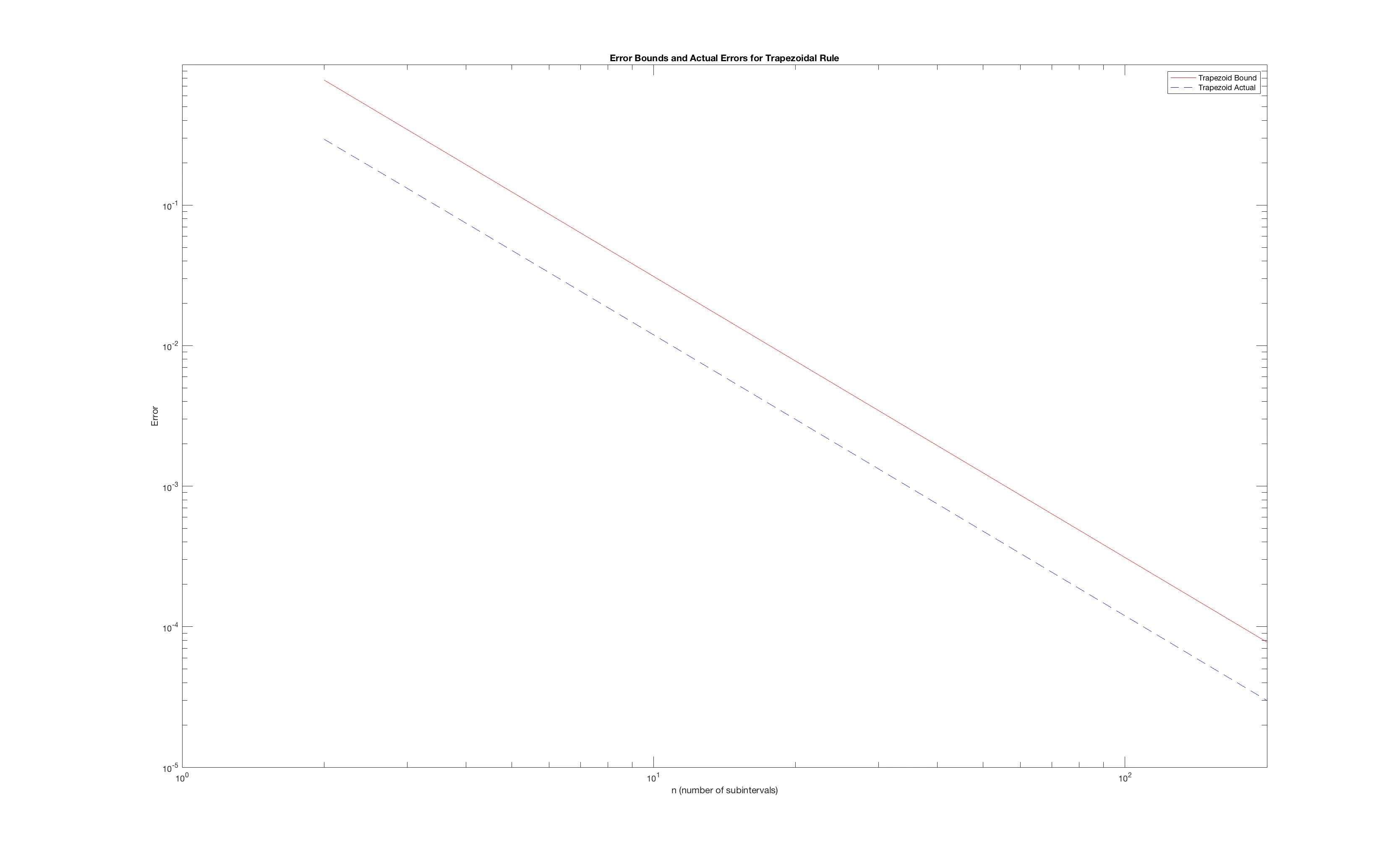
loglog(n_values, bounds_trap, 'r-', n_values, actual_errors_trap, 'b--');
legend('Trapezoid Bound', 'Trapezoid Actual');
title('Error Bounds and Actual Errors for Trapezoidal Rule');
xlabel('n (number of subintervals)');
ylabel('Error');yields
Simpson’s
The following:
f = @(x) exp(x) .* cos(x);
a = 0;
b = pi/2;
n_values = 2:2:200; % Simpson's rule requires an even number of intervals
tol = 1e-4;
exact_integral = integral(f, a, b);
% Initialize arrays to store the actual errors and theoretical error bounds
actual_errors_simp = zeros(size(n_values));
bounds_simp = zeros(size(n_values));
% Compute the fourth derivative for Simpson's rule error bound
max_f_4th = max(abs(exp(linspace(a, b, 1000)) .* (cos(linspace(a, b, 1000)) - 4.*sin(linspace(a, b, 1000)) - 6.*cos(linspace(a, b, 1000)) - 4.*sin(linspace(a, b, 1000)) + cos(linspace(a, b, 1000)))));
% Calculate errors and bounds for each n
for i = 1:length(n_values)
n = n_values(i);
% Simpson's rule calculations
approx_integral_simp = simpson(f, a, b, n);
actual_errors_simp(i) = abs(exact_integral - approx_integral_simp);
bounds_simp(i) = ((b - a)^5 / (180 * n^4)) * max_f_4th;
end
% Plot the error bounds and actual errors on a loglog plot
figure;
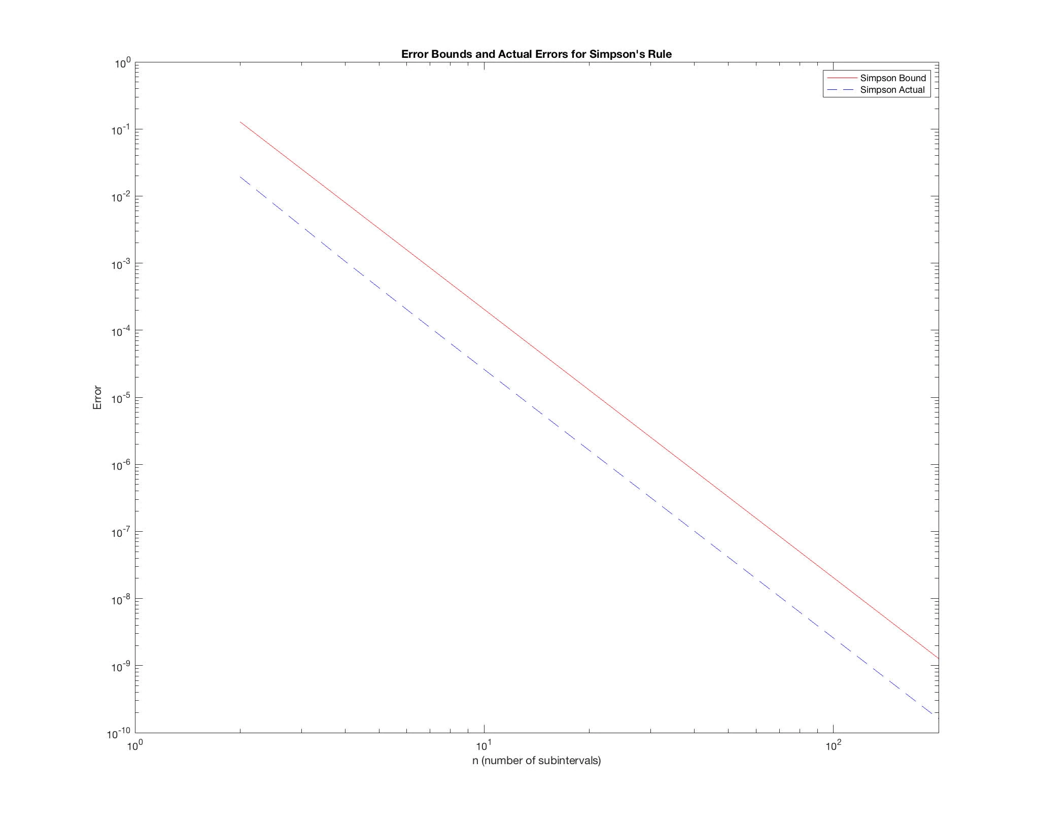
loglog(n_values, bounds_simp, 'r-', n_values, actual_errors_simp, 'b--');
legend('Simpson Bound', 'Simpson Actual');
title('Error Bounds and Actual Errors for Simpson''s Rule');
xlabel('n (number of subintervals)');
ylabel('Error');yields
d.
Trapezoidal
Error bound for theoretical is proportional to , therefore on the loglog the theoretical appears to be a straight lines with negative slope. Slope should be -2, because the error bound decreases with square of # n
The actual error observed also diminished as becomes larger. Similar to error bound, the actual error is expected to decrease with increase in n, but may decrease faster/slower. In loglog plot, it then appears to be straight line.
Simpson’s
Error bound for theoretical is proportional to , therefore on the loglog the theoretical appears to be a straight lines with negative slope.
The actual error observed when using Simpson’s rule also shows a rapid decrease with increasing . The actual error may decrease faster than the error bound predicts because the bound is a worst-case estimate. The true error often is less than this bound, especially for well-behaved functions.
The difference in slopes between the actual error curve and the theoretical error bound curve is expected. The theoretical curve represents the maximum possible error, not the exact error, which can be much less depending on how the function behaves within each subinterval.
The actual error may flatten as increases past a certain point. This is due to the limitations of numerical precision in Matlab.
Problem 4
function timeadd
% Define the sizes of the matrices
sizes = 500:100:1500;
times_addR = zeros(length(sizes), 1);
times_addC = zeros(length(sizes), 1);

% Time the functions and record the execution times
for i = 1:length(sizes)
  n = sizes(i);
  A = rand(n, n);
  B = rand(n, n);

  f_addR = @() addR(A, B);
  f_addC = @() addC(A, B);

  times_addR(i) = timeit(f_addR);
  times_addC(i) = timeit(f_addC);
end

% Perform least squares fitting to the model t = cn^2
X = [ones(length(sizes), 1), sizes'.^2];
crow_krow = X \ times_addR;
ccol_kcol = X \ times_addC;

% Output the constants
fprintf('crow: %e\n', crow_krow(1));
fprintf('krow: %e\n', crow_krow(2));
fprintf('ccol: %e\n', ccol_kcol(1));
fprintf('kcol: %e\n', ccol_kcol(2));

% Plot the results
figure;
loglog(sizes, times_addR, 'o-', 'DisplayName', 'addR');
hold on;
loglog(sizes, times_addC, 'o-', 'DisplayName', 'addC');
xlabel('Matrix Size (n)');
ylabel('Time (seconds)');
title('Time Complexity of Matrix Addition');
legend show;
grid on;
end

function C = addR(A, B)
[n, ~] = size(A);
C = zeros(n, n);
for i = 1:n
  C(i, :) = A(i, :) + B(i, :);
end
end

function C = addC(A, B)
[n, ~] = size(A);
C = zeros(n, n);
for j = 1:n
  C(:, j) = A(:, j) + B(:, j);
end
end
Yields
crow: -7.047139e-03
krow: 2.787915e-08
ccol: -4.545719e-04
kcol: 1.913233e-09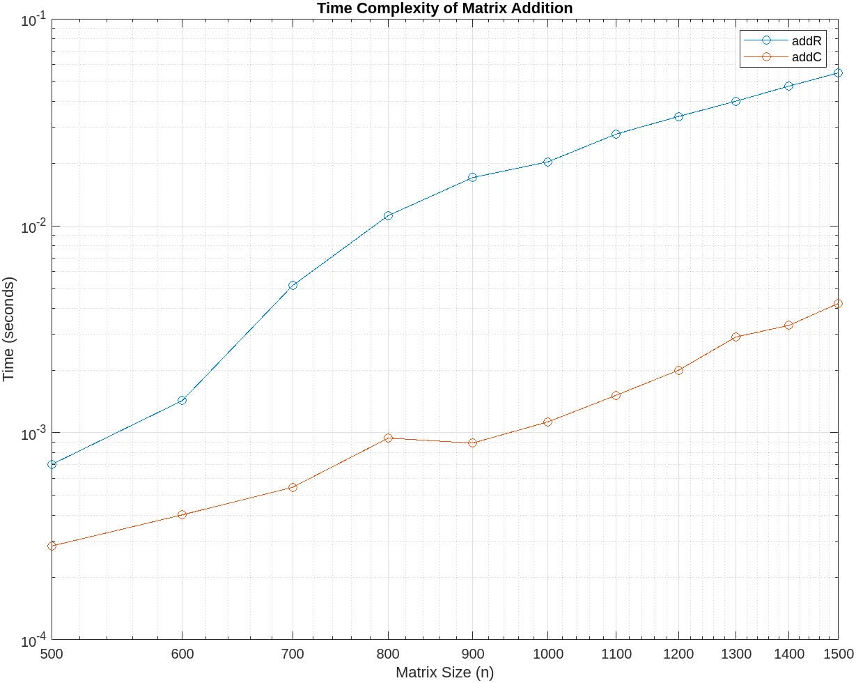
Reason for
- Overhead of function call: we include a lot of measurement noise in the function, so probably will increase system load and other process.
addRmemory access:addRis not optimal since MATLAB’s column-major order. Accessing elements row-wise can lead to cache misses and inefficient usage of memory bandwidth.- Added overheads, maybe associated with MATLAB’s JIT compilation, memory management.
- Polynomial fitting: LS model fits a polynomial of form . If error that increase with , then there is a leading overestimation of the quadratic term.
Problem 5
For each datapoint , compute the residual as
Sum of squared residuals
Or in this case is minimized
Or and
which results to and
and
Problem 6
a.
Or
# Given data
l_values = [7, 9.4, 12.3]  # l values
F_values = [2, 4, 6]       # F(l) values
l0 = 5.3                   # Unstretched length of the spring

# Calculate the numerator and denominator for the k value
numerator = sum([F * (l - l0) for F, l in zip(F_values, l_values)])
denominator = sum([(l - l0)**2 for l in l_values])

# Calculate k
k = numerator / denominator
b. Using the same logic with additional data, we get
# Additional measurements for part B
additional_l_values = [8.3, 11.3, 14.4, 15.9]  # Additional l values
additional_F_values = [3, 5, 8, 10]            # Additional F(l) values

# Combine old and new data points
all_l_values = l_values + additional_l_values
all_F_values = F_values + additional_F_values

# Calculate the numerator and denominator for the new k value
numerator_all = sum([F * (l - l0) for F, l in zip(all_F_values, all_l_values)])
denominator_all = sum([(l - l0)**2 for l in all_l_values])

# Calculate the new k using all data
k_all = numerator_all / denominator_all
To determine which constant k best fit the dataset, we calculate the sum of squares of residuals SSR using entire datasets
# Calculate the sum of squares of residuals for the original k and the new k
def sum_of_squares(k, l_values, F_values, l0):
    return sum([(k * (l - l0) - F)**2 for l, F in zip(l_values, F_values)])

# Sum of squares of residuals using k from part A for the whole data
SSR_k = sum_of_squares(k, all_l_values, all_F_values, l0)

# Sum of squares of residuals using k from part B for the whole data
SSR_k_all = sum_of_squares(k_all, all_l_values, all_F_values, l0)

SSR_k, SSR_k_all
This yield SSR from A is approx. 0.9062, whereas from part B is approx 0.8962.
The lower the better here, which means part B is a better fit to the entire data comparing to part A.