ml optimization softmax softmax(y) i = e y i ∑ i e y i \text{softmax(y)}_i = \frac{e^{y_i}}{\sum_{i} e^{y_i}} softmax(y) i = ∑ i e y i e y i where y ∈ R k y \in \mathbb{R}^k y ∈ R k
exp()
Usually a lot better comparing to 2**t simply for
For ARM the design specially
pseudocode-exp-fexpa.cpp // Pseudocode representing the computation flow: float32x4_t exp_sve2 ( float32x4_t x ) { // Step 1: Range reduction // N = round(x * log2(e)) // r = x - N * ln(2) [reduced argument]
// Step 2: FEXPA instruction provides 2^N approximation // In hardware: FEXPA Z0.S, Z1.S float32x4_t exp_approx ; // Result of FEXPA
// Step 3: Polynomial evaluation for exp(r) // Typically uses Horner's method with reduced precision // coefficients since we're starting with a good approximation float32x4_t exp_r = evaluate_polynomial ( r );
// Step 4: Combine results return exp_approx * exp_r ; } Advantages of FEXPA:
single instruction latency for initial approximation
vectorized ops for batch processing
On GPU we can utilise bit-shift 1<<x or CUDA’s exp2
Optimization in llama.cpp:
RoPE (
sigmoid sigmoid ( x ) = 1 1 + e − x \text{sigmoid}(x) = \frac{1}{1+e^{-x}} sigmoid ( x ) = 1 + e − x 1 ReLU FFN ( x , W 1 , W 2 , b 1 , b 2 ) = m a x ( 0 , x W 1 + b 1 ) W 2 + b 2 \text{FFN}(x, W_{1}, W_{2}, b_{1}, b_{2}) = max(0, xW_{1}+b_{1})W_{2} + b_{2} FFN ( x , W 1 , W 2 , b 1 , b 2 ) = ma x ( 0 , x W 1 + b 1 ) W 2 + b 2 A version in T5 without bias:
FFN ReLU ( x , W 1 , W 2 ) = m a x ( x W 1 , 0 ) W 2 \text{FFN}_\text{ReLU}(x,W_{1},W_{2}) = max(xW_{1},0)W_{2} FFN ReLU ( x , W 1 , W 2 ) = ma x ( x W 1 , 0 ) W 2 Swish
f ( x ) = x ⋅ sigmoid ( β x ) ∵ β : constant parameter f(x) = x \cdotp \text{sigmoid}(\beta x)
\\
\because \beta : \text{ constant parameter} f ( x ) = x ⋅ sigmoid ( β x ) ∵ β : constant parameter Gated Linear Units and Variants
component-wise product of two linear transformations of the inputs, one of which is sigmoid-activated.
GLU ( x , W , V , b , c ) = σ ( x W + b ) ⊗ ( x V + c ) Bilinear ( x , W , V , b , c ) = ( x W + b ) ⊗ ( x V + c ) \begin{aligned}
\text{GLU}(x,W,V,b,c) &= \sigma(xW+b) \otimes (xV+c) \\
\text{Bilinear}(x,W,V,b,c) &= (xW+b) \otimes (xV+c)
\end{aligned} GLU ( x , W , V , b , c ) Bilinear ( x , W , V , b , c ) = σ ( x W + b ) ⊗ ( x V + c ) = ( x W + b ) ⊗ ( x V + c ) GLU in other variants:
ReGLU ( x , W , V , b , c ) = max ( 0 , x W + b ) ⊗ ( x V + c ) GEGLU ( x , W , V , b , c ) = GELU ( x W + b ) ⊗ ( x V + c ) SwiGLU ( x , W , V , b , c ) = Swish β ( x W + b ) ⊗ ( x V + c ) \begin{aligned}
\text{ReGLU}(x,W,V,b,c) &= \max(0, xW+b) \otimes (xV+c) \\
\text{GEGLU}(x,W,V,b,c) &= \text{GELU}(xW+b) \otimes (xV+c) \\
\text{SwiGLU}(x,W,V,b,c) &= \text{Swish}_\beta(xW+b) \otimes (xV+c)
\end{aligned} ReGLU ( x , W , V , b , c ) GEGLU ( x , W , V , b , c ) SwiGLU ( x , W , V , b , c ) = max ( 0 , x W + b ) ⊗ ( x V + c ) = GELU ( x W + b ) ⊗ ( x V + c ) = Swish β ( x W + b ) ⊗ ( x V + c ) FFN for transformers layers would become:
FFN GLU ( x , W , V , W 2 ) = ( σ ( x W ) ⊗ x V ) W 2 FFN Bilinear ( x , W , V , W 2 ) = ( x W ⊗ x V ) W 2 FFN ReGLU ( x , W , V , W 2 ) = ( max ( 0 , x W ) ⊗ x V ) W 2 FFN GEGLU ( x , W , V , W 2 ) = ( GELU ( x W ) ⊗ x V ) W 2 FFN SwiGLU ( x , W , V , W 2 ) = ( Swish β ( x W ) ⊗ x V ) W 2 \begin{aligned}
\text{FFN}_\text{GLU}(x,W,V,W_{2}) &= (\sigma (xW) \otimes xV)W_{2} \\
\text{FFN}_\text{Bilinear}(x,W,V,W_{2}) &= (xW \otimes xV)W_{2} \\
\text{FFN}_\text{ReGLU}(x,W,V,W_{2}) &= (\max(0, xW) \otimes xV)W_{2} \\
\text{FFN}_\text{GEGLU}(x,W,V,W_{2}) &= (\text{GELU}(xW) \otimes xV)W_{2} \\
\text{FFN}_\text{SwiGLU}(x,W,V,W_{2}) &= (\text{Swish}_\beta(xW) \otimes xV)W_{2}
\end{aligned} FFN GLU ( x , W , V , W 2 ) FFN Bilinear ( x , W , V , W 2 ) FFN ReGLU ( x , W , V , W 2 ) FFN GEGLU ( x , W , V , W 2 ) FFN SwiGLU ( x , W , V , W 2 ) = ( σ ( x W ) ⊗ x V ) W 2 = ( x W ⊗ x V ) W 2 = ( max ( 0 , x W ) ⊗ x V ) W 2 = ( GELU ( x W ) ⊗ x V ) W 2 = ( Swish β ( x W ) ⊗ x V ) W 2 note : reduce number of hidden units d ff d_\text{ff} d ff W W W V V V W 2 W_{2} W 2 2 3 \frac{2}{3} 3 2
JumpReLU
J ( z ) ≔ z H ( z − κ ) = { 0 if z ≤ κ z if z > κ J(z) \coloneqq z H(z - \kappa) = \begin{cases} 0 & \text{if } z \leq \kappa \\ z & \text{if } z > \kappa \end{cases} J ( z ) : = zH ( z − κ ) = { 0 z if z ≤ κ if z > κ
momentum See also
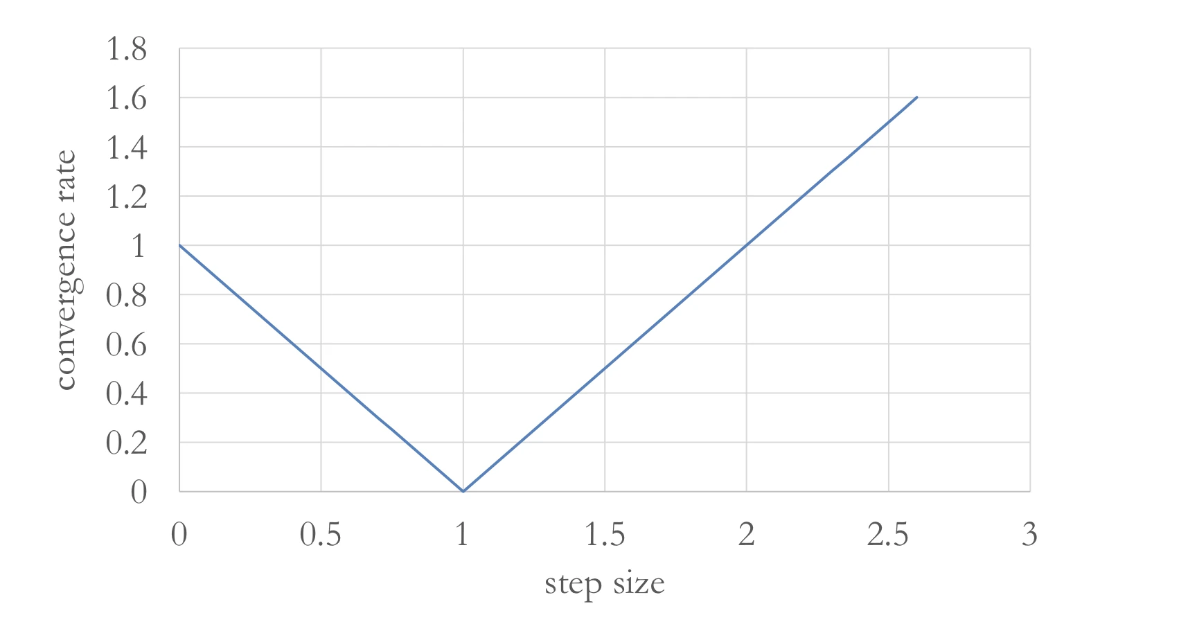
In the case of quadratic function: f ( x ) = 1 2 x 2 f(x) = \frac{1}{2} x^2 f ( x ) = 2 1 x 2 x t + 1 = x t − α x t = ( 1 − α ) x t x_{t+1} = x_t - \alpha x_t = (1-\alpha)x_t x t + 1 = x t − α x t = ( 1 − α ) x t
Think of convergence rate
∣ x t + 1 − 0 ∣ = ∣ 1 − α ∣ ∣ x t − 0 ∣ \mid x_{t+1} - 0 \mid = \mid 1 - \alpha \mid \mid x_t - 0 \mid ∣ x t + 1 − 0 ∣=∣ 1 − α ∣∣ x t − 0 ∣ If we set different curvature (f ( x ) = 2 x 2 f(x) = 2x^2 f ( x ) = 2 x 2 x t + 1 = x t − 4 α x t = ( 1 − 4 α ) x t x_{t+1} = x_t - 4 \alpha x_t = (1-4 \alpha)x_t x t + 1 = x t − 4 α x t = ( 1 − 4 α ) x t
step size depends on curvature for one-dimensional quadratics
more curvature means smaller ideal step size
how would this play for general quadratics?
for PSD symmetric A A A
f ( x ) = 1 2 x T A x f(x) = \frac{1}{2} x^T Ax f ( x ) = 2 1 x T A x with gradient descent has update step
x t + 1 = x t − α A x t = ( I − α A ) x t x_{t+1} = x_t - \alpha A x_t = (I - \alpha A)x_t x t + 1 = x t − α A x t = ( I − α A ) x t convergence rate would be
max x ∥ ( I − α A ) x ∥ ∥ x ∥ = max x 1 ∥ x ∥ ∥ ( I − α ∑ i = 1 n λ i u i u i T ) x ∥ = max x ∥ ∑ i = 1 n ( 1 − α λ i ) u i u i T x ∥ ∥ ∑ i = 1 n u i u i T x ∥ = m a x i ∣ 1 − α λ i ∣ = m a x ( 1 − α λ min , α λ max − 1 ) \begin{aligned}
\max_{x} \frac{\|(I - \alpha A)x\|}{\|x\|} &= \max_{x} \frac{1}{\|x\|} \left\| \left( I - \alpha \sum_{i=1}^{n} \lambda_i u_i u_i^T \right) x \right\| \\[8pt]
&= \max_{x} \frac{\|\sum_{i=1}^{n} (1- \alpha \lambda_i) u_i u_i^T x\|}{\|\sum_{i=1}^{n} u_i u_i^T x\|} \\
&= max_i \mid 1- \alpha \lambda_i \mid \\
&=max(1-\alpha \lambda_{\text{min}}, \alpha \lambda_{\text{max}} - 1)
\end{aligned} x max ∥ x ∥ ∥ ( I − α A ) x ∥ = x max ∥ x ∥ 1 ( I − α i = 1 ∑ n λ i u i u i T ) x = x max ∥ ∑ i = 1 n u i u i T x ∥ ∥ ∑ i = 1 n ( 1 − α λ i ) u i u i T x ∥ = ma x i ∣ 1 − α λ i ∣ = ma x ( 1 − α λ min , α λ max − 1 )
optimal value occurs when
1 − α λ min = α λ max − 1 ⇒ α = 2 λ max + λ min 1 - \alpha \lambda_{\text{min}} = \alpha \lambda_{\text{max}} - 1 \Rightarrow \alpha = \frac{2}{\lambda_{\text{max}} + \lambda_{\text{min}}} 1 − α λ min = α λ max − 1 ⇒ α = λ max + λ min 2 with rate
λ max − λ min λ max + λ min \frac{\lambda_{\text{max}} - \lambda_{\text{min}}}{\lambda_{\text{max}} + \lambda_{\text{min}}} λ max + λ min λ max − λ min
We denote κ = λ max λ min \kappa = \frac{\lambda_{\text{max}}}{\lambda_{\text{min}}} κ = λ min λ max condition number of matrix A
Problems with larger condition numbers converge slower.
Intuitively these are problems that are highly curved in some directions, but flat others
Polyak abbreviation: “heavy ball method”
idea: add an extra momentum term to gradient descent
x t + 1 = x t − α ∇ f ( x t ) + β ( x t − x t − 1 ) x_{t+1} = x_t - \alpha \nabla f(x_t) + \beta (x_t - x_{t-1}) x t + 1 = x t − α ∇ f ( x t ) + β ( x t − x t − 1 ) tl/dr: if current gradient step is in same direction as previous step, then move a little further in the same direction
momentum for 1D quadratics
f ( x ) = λ 2 x 2 f(x) = \frac{\lambda}{2} x^{2} f ( x ) = 2 λ x 2 momentum GD gives
x t + 1 = x t − α λ x t + β ( x t − x t − 1 ) = ( 1 + β − α λ ) x t − β x t − 1 \begin{aligned}
x_{t+1} &= x_t - \alpha \lambda x_t + \beta (x_t - x_{t-1}) \\
&= (1+\beta - \alpha \lambda) x_t - \beta x_{t-1}
\end{aligned} x t + 1 = x t − α λ x t + β ( x t − x t − 1 ) = ( 1 + β − α λ ) x t − β x t − 1 characterizing momentum:
start with x t + 1 = ( 1 + β − α λ ) x t − β x t − 1 x_{t+1} = (1+\beta -\alpha \lambda) x_t - \beta x_{t-1} x t + 1 = ( 1 + β − α λ ) x t − β x t − 1
trick: let x t = β t / 2 z t x_t = \beta^{t/2}z_t x t = β t /2 z t
z t + 1 = 1 + β − α λ β z t − z t − 1 z_{t+1} = \frac{1 + \beta - \alpha \lambda}{\sqrt{\beta}} z_t - z_{t-1} z t + 1 = β 1 + β − α λ z t − z t − 1 let u = 1 + β − α λ 2 β u = \frac{1+\beta -\alpha \lambda}{2 \sqrt{\beta}} u = 2 β 1 + β − α λ
z t + 1 = 2 u z t − z t − 1 z_{t+1} = 2 u z_t - z_{t-1} z t + 1 = 2 u z t − z t − 1 degree-t \textbf{t} t u \textbf{u} u
Nesterov See also
idea:
first take a step in the direction of accumulated momentum
computes gradient at “lookahead” position,
make the update using this gradient.
For a parameter vector θ \theta θ
v t = μ v t − 1 + ∇ L ( θ t + μ v t − 1 ) θ t + 1 = θ t − α v t \begin{aligned}
v_t &= \mu v_{t-1} + \nabla L(\theta_t + \mu v_{t-1}) \\
\theta_{t+1} &= \theta_t - \alpha v_t
\end{aligned} v t θ t + 1 = μ v t − 1 + ∇ L ( θ t + μ v t − 1 ) = θ t − α v t
Achieves better convergence rates
function type gradient descent Nesterove AG Smooth θ ( 1 T ) \theta(\frac{1}{T}) θ ( T 1 ) θ ( 1 T 2 ) \theta(\frac{1}{T^{2}}) θ ( T 2 1 ) Smooth & Strongly Convex θ ( exp ( − T κ ) ) \theta(\exp (-\frac{T}{\kappa})) θ ( exp ( − κ T )) θ ( exp − T κ ) \theta(\exp -\frac{T}{\sqrt{\kappa}}) θ ( exp − κ T )
optimal assignments for parameters
α = 1 λ max , β = κ − 1 κ + 1 \alpha = \frac{1}{\lambda_{\text{max}}}, \beta = \frac{\sqrt{\kappa} - 1}{\sqrt{\kappa} + 1} α = λ max 1 , β = κ + 1 κ − 1
Bibliographie Abdelkhalik, H., Arafa, Y., Santhi, N., & Badawy, A.-H. (2022). Demystifying the Nvidia Ampere Architecture through Microbenchmarking and Instruction-level Analysis . arXiv preprint arXiv:2208.11174 Erichson, N. B., Yao, Z., & Mahoney, M. W. (2019). JumpReLU: A Retrofit Defense Strategy for Adversarial Attacks . arXiv preprint arXiv:1904.03750 Rajamanoharan, S., Lieberum, T., Sonnerat, N., Conmy, A., Varma, V., Kramár, J., & Nanda, N. (2024). Jumping Ahead: Improving Reconstruction Fidelity with JumpReLU Sparse Autoencoders . arXiv preprint arXiv:2407.14435 Ramachandran, P., Zoph, B., & Le, Q. V. (2017). Searching for Activation Functions . arXiv preprint arXiv:1710.05941 Shazeer, N. (2020). GLU Variants Improve Transformer . arXiv preprint arXiv:2002.05202 Su, J., Lu, Y., Pan, S., Murtadha, A., Wen, B., & Liu, Y. (2023). RoFormer: Enhanced Transformer with Rotary Position Embedding . arXiv preprint arXiv:2104.09864