System response We will consider first-order and second-order system
first-order systems, time constant "\\usepackage{tikz}\n\\usetikzlibrary{positioning}\n\n\\begin{document}\n\\begin{tikzpicture}[auto, node distance=2cm, >=latex]\n\n% Nodes\n\\node[draw, rectangle, minimum width=3cm, minimum height=1.5cm] (block) {$\\frac{a}{s + a}$};\n\\node[left=1.5cm of block] (input) {$X(s) = \\frac{1}{s}$};\n\\node[right=1.5cm of block] (output) {$Y(s)$};\n\\node[above=0.5cm of block] (G) {$G(s)$};\n\n% Arrows\n\\draw[->] (input) -- (block);\n\\draw[->] (block) -- (output);\n\n\\end{tikzpicture}\n\\end{document}" a s + a X ( s ) = 1 s Y ( s ) G ( s ) source code Output of a general first-order system is
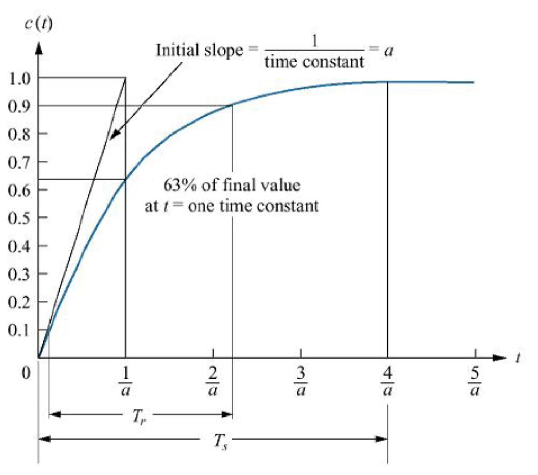
Y ( s ) = X ( s ) G ( s ) = a s ( s + a ) Y(s) = X(s)G(s) = \frac{a}{s(s+a)} Y ( s ) = X ( s ) G ( s ) = s ( s + a ) a thus the time domain output is y ( t ) = 1 − e − a t y(t) = 1 - e^{-at} y ( t ) = 1 − e − a t
usually, t = 1 a t=\frac{1}{a} t = a 1 y ( t ) = 0.63 y(t) = 0.63 y ( t ) = 0.63
response in time domain
T r T_r T r
for first order: T r = 2.2 a T_r = \frac{2.2}{a} T r = a 2.2
T s T_s T s
for first order: T s = 4 a T_s = \frac{4}{a} T s = a 4
second-order systems general order system:
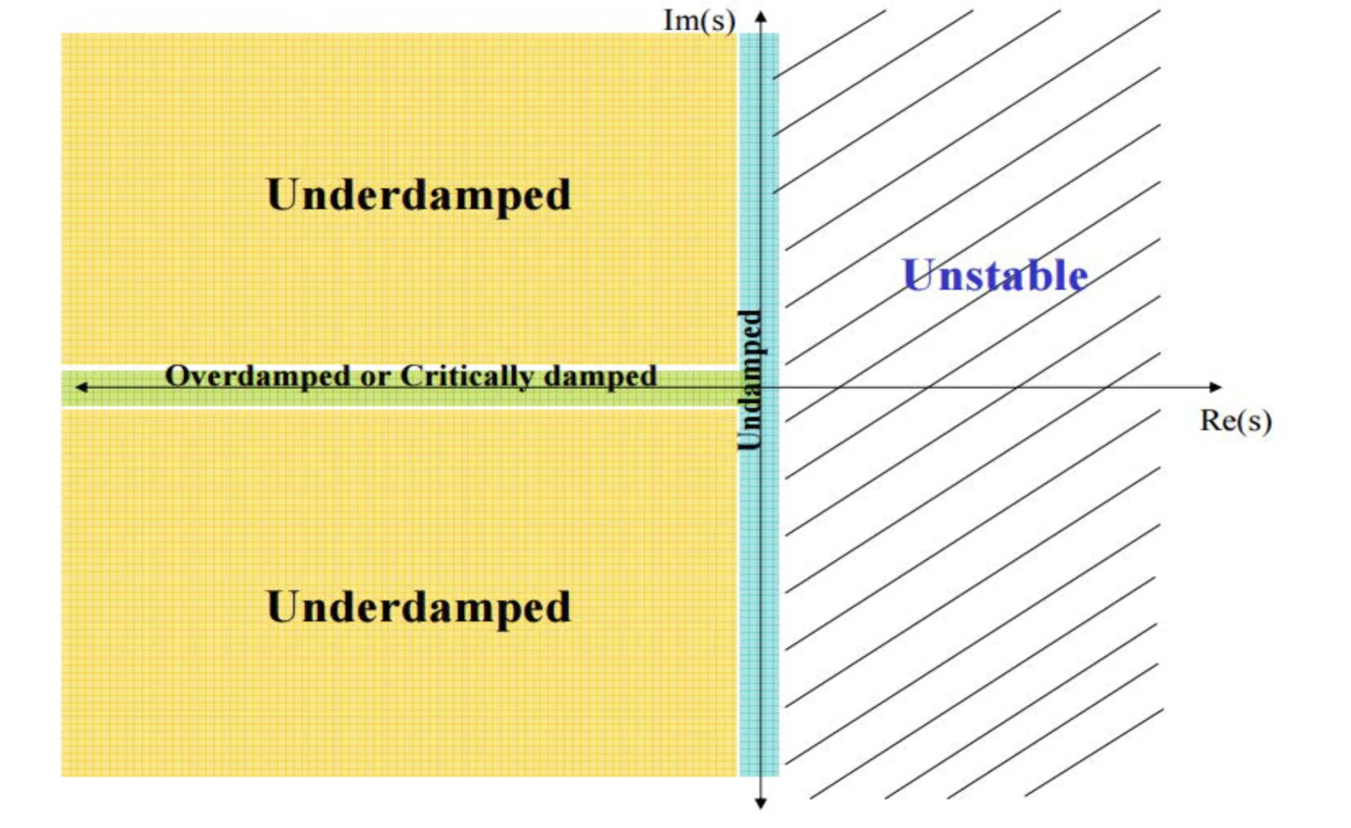
G ( s ) = b s 2 + a s + b G(s) = \frac{b}{s^{2}+as +b} G ( s ) = s 2 + a s + b b Thus the pole for this system:
s 1 , s 2 = − a + a 2 − 4 b 2 s_{1},s_{2}= \frac{-a + \sqrt{a^2 - 4b}}{2} s 1 , s 2 = 2 − a + a 2 − 4 b natural frequency happens when a = 0 a=0 a = 0
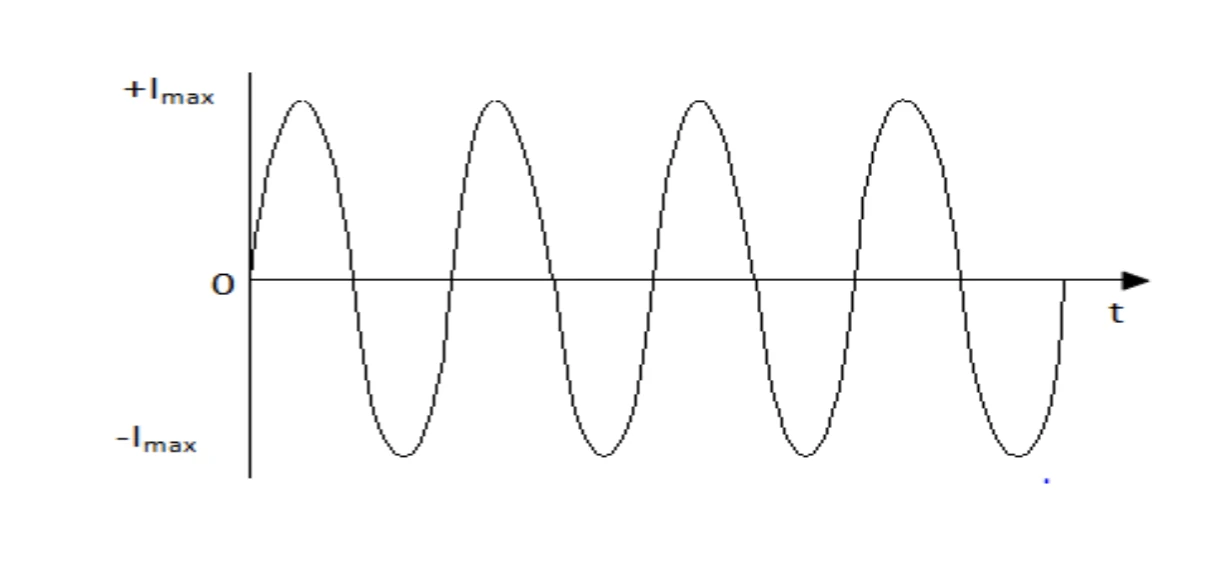
The transfer function is G ( s ) = b s 2 + b G(s)=\frac{b}{s^{2}+b} G ( s ) = s 2 + b b ± j w \pm jw ± j w
w n = b w_n = \sqrt{b} w n = b
in a sense, this is the undamped case:
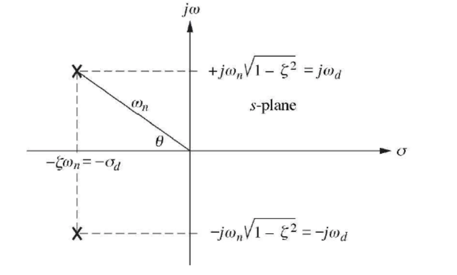
damping coefficient complex poles has real part σ = − a 2 \sigma = -\frac{a}{2} σ = − 2 a
damping ratio is defined as:
ζ = exponential decay frequency natural frequency = ∣ σ ∣ w n \zeta = \frac{\text{exponential decay frequency}}{\text{natural frequency}} = \frac{|\sigma|}{w_n} ζ = natural frequency exponential decay frequency = w n ∣ σ ∣
So that a = 2 ζ w n a = 2 \zeta w_n a = 2 ζ w n
general second order G ( s ) = w n 2 s 2 + 2 ζ w n s + w n 2 s 1 , s 2 = − ζ w n ± w n ζ 2 − 1 \begin{aligned}
G(s) &= \frac{w_n^2}{s^2 + 2 \zeta w_n s + w_n^2} \\[12pt]
s_{1},s_{2} &= - \zeta w_n \pm w_n \sqrt{\zeta^2 - 1}
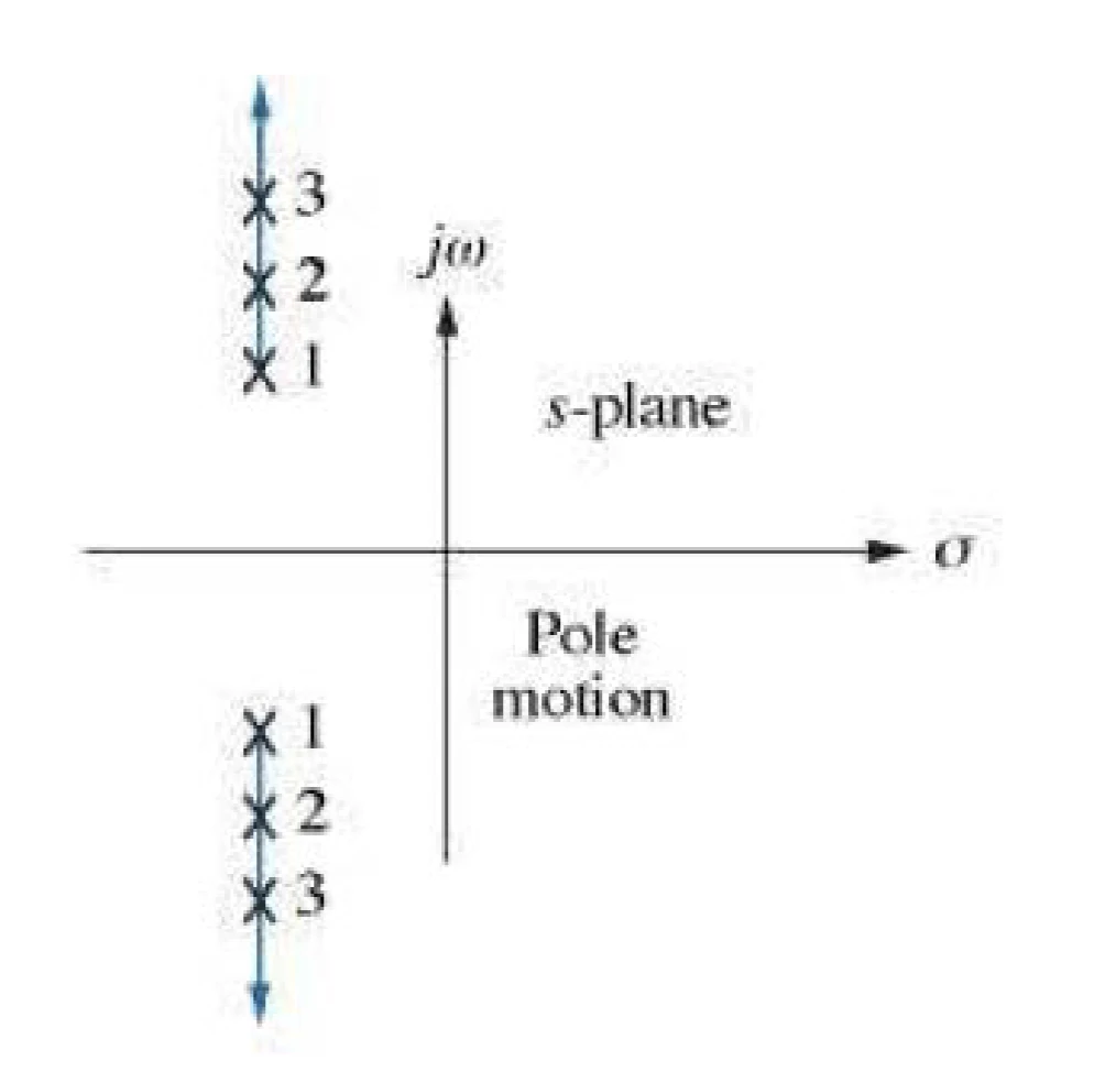
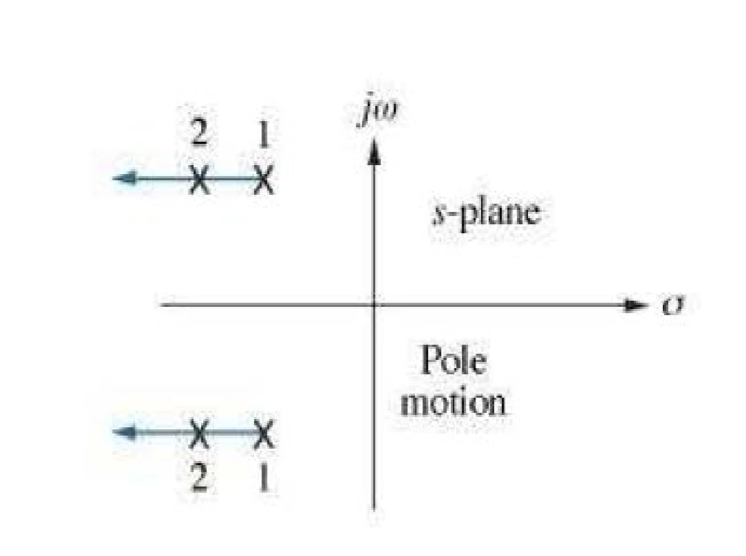
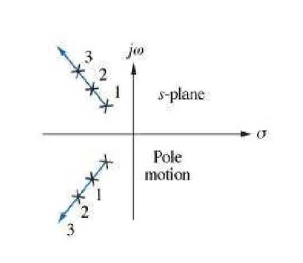
\end{aligned} G ( s ) s 1 , s 2 = s 2 + 2 ζ w n s + w n 2 w n 2 = − ζ w n ± w n ζ 2 − 1 observations Condition Poles pole type Damping Ratio (ζ \zeta ζ Natural Response c ( t ) c(t) c ( t ) Undamped ± j ω n \pm j \omega_n ± j ω n imaginary ζ = 0 \zeta = 0 ζ = 0 A cos ( ω n t − φ ) A \cos (\omega_n t - \varphi) A cos ( ω n t − φ ) Underdamped ω d ± j ω d \omega_d \pm j \omega_d ω d ± j ω d complex 0 < ζ < 1 0 < \zeta < 1 0 < ζ < 1 A e ( − σ d ) t cos ( ω d t − φ ) A e^{(-\sigma_d)t} \cos (\omega_d t - \varphi) A e ( − σ d ) t cos ( ω d t − φ ) w d = w n 1 − ζ 2 w_d = w_n \sqrt{1- \zeta^2} w d = w n 1 − ζ 2 critically damped σ 1 \sigma_1 σ 1 real ζ = 1 \zeta = 1 ζ = 1 K t e σ 1 t K t e^{\sigma_1 t} K t e σ 1 t overdamped σ 1 σ 2 \sigma_1 \quad \sigma_2 σ 1 σ 2 real ζ > 1 \zeta > 1 ζ > 1 K ( e σ 1 t + e σ 2 t ) K (e^{\sigma_1 t} + e^{\sigma_2 t}) K ( e σ 1 t + e σ 2 t )
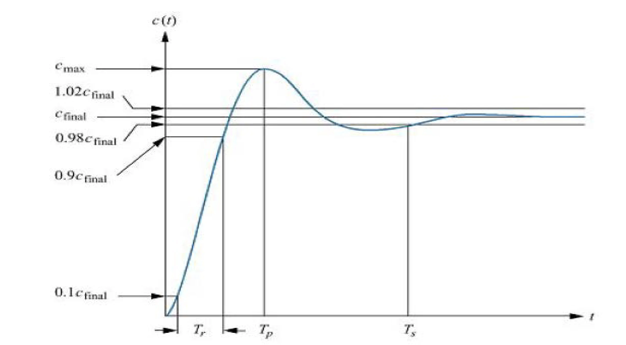
underdamped second-order step response Transfer function C ( s ) C(s) C ( s )
C ( s ) = w n 2 s ( s 2 + 2 ζ w n s + w n 2 ) C(s) = \frac{w_n^2}{s(s^2 + 2 \zeta w_n s + w_n^2)} C ( s ) = s ( s 2 + 2 ζ w n s + w n 2 ) w n 2 response in time-domain via inverse Laplace transform:
c ( t ) = 1 − 1 1 − ζ 2 e − ζ w n t cos ( 1 − ζ 2 ω n t + φ ) c(t) = 1 - \frac{1}{\sqrt{1- \zeta^2}} e^{- \zeta w_n t} \cos (\sqrt{1- \zeta^2}\omega_n t + \varphi) c ( t ) = 1 − 1 − ζ 2 1 e − ζ w n t cos ( 1 − ζ 2 ω n t + φ ) where φ = tan − 1 ( ζ 1 − ζ 2 ) \varphi = \tan^{-1} (\frac{\zeta}{\sqrt{1-\zeta^2}}) φ = tan − 1 ( 1 − ζ 2 ζ )
peak time T p T_p T p time required to reach the first or maximum peak
T p = π ω n 1 − ζ 2 T_p = \frac{\pi}{\omega_n \sqrt{1-\zeta^2}} T p = ω n 1 − ζ 2 π percent overshoot %OS (percent overshoot) % O S = e ζ π / 1 − ζ 2 × 100 % \%OS = e^{\zeta \pi / \sqrt{1-\zeta^2}} \times 100 \% % OS = e ζ π / 1 − ζ 2 × 100% or in terms of damping ratio ζ \zeta ζ
ζ = − ln %OS 100 π 2 + ln 2 ( %OS 100 ) \zeta = \frac{-\ln \frac{\text{\%OS}}{100}}{\sqrt{\pi^2 + \ln^2(\frac{\text{\%OS}}{100})}} ζ = π 2 + ln 2 ( 100 %OS ) − ln 100 %OS relations to poles G ( s ) = w n 2 s 2 + 2 ζ w n s + w n 2 s 1 , s 2 = − ζ w n ± w n ζ 2 − 1 T p = π ω n 1 − ζ 2 T s ≅ 4 ζ ω n \begin{aligned}
G(s) &= \frac{w_n^2}{s^2 + 2 \zeta w_n s + w_n^2} \\[12pt]
s_{1},s_{2} &= - \zeta w_n \pm w_n \sqrt{\zeta^2 - 1} \\[8pt]
T_p &= \frac{\pi}{\omega_n \sqrt{1-\zeta^2}} \\
T_s &\cong \frac{4}{\zeta \omega_n}
\end{aligned} G ( s ) s 1 , s 2 T p T s = s 2 + 2 ζ w n s + w n 2 w n 2 = − ζ w n ± w n ζ 2 − 1 = ω n 1 − ζ 2 π ≅ ζ ω n 4 figure 1 : poles of second-order underdamped system same envelope "\\usepackage{tikz}\n\\usepackage{pgfplots}\n\\pgfplotsset{compat=1.16}\n\n\\begin{document}\n\\begin{tikzpicture}\n \\begin{axis}[\n width=12cm, height=8cm,\n xlabel={$t$ (time)},\n ylabel={Amplitude},\n grid=major,\n legend style={at={(0.5,1.1)}, anchor=north, legend columns=-1},\n xmin=0, xmax=10,\n ymin=-1.2, ymax=1.2\n ]\n % First Transfer Function (Sinusoidal)\n \\addplot[blue, thick, samples=100, domain=0:10]\n {exp(-0.1*x)*sin(deg(2*pi*0.5*x))};\n\n % Second Transfer Function (Envelope with Different Frequency)\n \\addplot[red, dashed, thick, samples=100, domain=0:10]\n {exp(-0.1*x)*sin(deg(2*pi*0.8*x))};\n\n % Envelope (Exponential Decay)\n \\addplot[black, dotted, thick, samples=100, domain=0:10]\n {exp(-0.1*x)};\n\n \\addplot[black, dotted, thick, samples=100, domain=0:10]\n {-exp(-0.1*x)};\n \\end{axis}\n\\end{tikzpicture}\n\\end{document}" 0 1 2 3 4 5 6 7 8 9 10 ¡ 1 ¡ 0 : 5 0 0 : 5 1 t (time) Amplitude source code same frequency "\\usepackage{tikz}\n\\usepackage{pgfplots}\n\\pgfplotsset{compat=1.16}\n\n\\begin{document}\n\\begin{tikzpicture}\n \\begin{axis}[\n width=12cm, height=8cm,\n xlabel={$t$ (time)},\n ylabel={Amplitude},\n grid=major,\n legend style={at={(0.5,1.1)}, anchor=north, legend columns=-1},\n xmin=0, xmax=10,\n ymin=-3, ymax=3\n ]\n % First Transfer Function (Higher Amplitude)\n \\addplot[blue, thick, samples=100, domain=0:10]\n {2*sin(deg(2*pi*0.5*x))};\n\n % Second Transfer Function (Lower Amplitude)\n \\addplot[red, dashed, thick, samples=100, domain=0:10]\n {1*sin(deg(2*pi*0.5*x))};\n \\end{axis}\n\\end{tikzpicture}\n\\end{document}" 0 1 2 3 4 5 6 7 8 9 10 ¡ 3 ¡ 2 ¡ 1 0 1 2 3 t (time) Amplitude source code same overshoot "\\usepackage{tikz}\n\\usepackage{pgfplots}\n\\pgfplotsset{compat=1.16}\n\n\\begin{document}\n\\begin{tikzpicture}\n \\begin{axis}[\n width=12cm, height=8cm,\n xlabel={Time $t$},\n ylabel={Response},\n grid=major,\n legend style={at={(0.5,1.1)}, anchor=north, legend columns=-1},\n xmin=0, xmax=10,\n ymin=0, ymax=2\n ]\n % First System Response\n \\addplot[blue, thick, samples=200, domain=0:10]\n {1 - exp(-0.5*x)*(cos(deg(2*pi*0.5*x)) + 0.1*sin(deg(2*pi*0.5*x)))};\n\n % Second System Response (Same Overshoot, Different Natural Frequency)\n \\addplot[red, dashed, thick, samples=200, domain=0:10]\n {1 - exp(-1*x)*(cos(deg(2*pi*1*x)) + 0.05*sin(deg(2*pi*1*x)))};\n\n % Reference Line for Steady-State Response\n \\addplot[black, dotted, thick] coordinates {(0,1) (10,1)};\n \\end{axis}\n\\end{tikzpicture}\n\\end{document}" 0 1 2 3 4 5 6 7 8 9 10 0 0 : 5 1 1 : 5 2 Time t Resp onse source code