whirlwind tour, initial exploration, glossary
The subfield of alignment that delves into reverse engineering of a neural network, especially LLMs
To attack the curse of dimensionality, the question remains: how do we hope to understand a function over such a large space, without an exponential amount of time? 1
Topics:
open problems
- differentiate between “reverse engineering” versus “concept-based”
- reverse engineer:
- decomposition → hypotheses → validation
- Decomposition via dimensionality reduction
- decomposition → hypotheses → validation
- drawbacks with SDL:
- SDL reconstruction error are way too high (Rajamanoharan et al., 2024, p. see section 2.3)
- SDL assumes linear representation hypothesis against non-linear feature space.
- SDL leaves feature geometry unexplained
- reverse engineer:
inference
Application in the wild: Goodfire and Transluce
How we would do inference with SAE?
Quick 🧵 and some of quick introspection into how they might run inference https://t.co/1N3JrxFHSp
— aaron (@aarnphm_) 25 septembre 2024
idea: treat SAEs as a logit bias, similar to guided decoding
steering
refers to the process of manually modifying certain activations and hidden state of the neural net to influence its outputs
For example, the following is a toy example of how a decoder-only transformers (i.e: GPT-2) generate text given the prompt “The weather in California is”
flowchart LR
  A[The weather in California is] --> B[H0] --> D[H1] --> E[H2] --> C[... hot]
To steer to model, we modify layers with certain features amplifier with scale 20 (called it )2
flowchart LR
  A[The weather in California is] --> B[H0] --> D[H1] --> E[H3] --> C[... cold]
One usually use techniques such as sparse autoencoders to decompose model activations into a set of interpretable features.
For feature ablation, we observe that manipulation of features activation can be strengthened or weakened to directly influence the model’s outputs
example: Panickssery et al. (2024) uses contrastive activation additions to steer Llama 2
contrastive activation additions
intuition: using a contrast pair for steering vector additions at certain activations layers
Uses mean difference which produce difference vector similar to PCA:
Given a dataset of prompt with positive completion and negative completion , we calculate mean-difference at layer as follow:
implication
by steering existing learned representations of behaviors, CAA results in better out-of-distribution generalization than basic supervised finetuning of the entire model.
superposition hypothesis
tl/dr
phenomena when a neural network represents more than features in a -dimensional space
Linear representation of neurons can represent more features than dimensions. As sparsity increases, model use superposition to represent more features than dimensions.
neural networks “want to represent more features than they have neurons”.
When features are sparsed, superposition allows compression beyond what linear model can do, at a cost of interference that requires non-linear filtering.
reasoning: “noisy simulation”, where small neural networks exploit feature sparsity and properties of high-dimensional spaces to approximately simulate much larger much sparser neural networks
In a sense, superposition is a form of lossy compression
importance
-
sparsity: how frequently is it in the input?
-
importance: how useful is it for lowering loss?
over-complete basis
reasoning for the set of directions 3
features
A property of an input to the model
When we talk about features (Elhage et al., 2022, p. see “Empirical Phenomena”), the theory building around several observed empirical phenomena:
- Word Embeddings: have direction which corresponding to semantic properties (Mikolov et al., 2013). For
example:
V(king) - V(man) = V(monarch) - Latent space: similar vector arithmetics and interpretable directions have also been found in generative adversarial network.
We can define features as properties of inputs which a sufficiently large neural network will reliably dedicate a neuron to represent (Elhage et al., 2022, p. see “Features as Direction”)
ablation
refers to the process of removing a subset of a model’s parameters to evaluate its predictions outcome.
idea: deletes one activation of the network to see how performance on a task changes.
- zero ablation or pruning: Deletion by setting activations to zero
- mean ablation: Deletion by setting activations to the mean of the dataset
- random ablation or resampling
residual stream
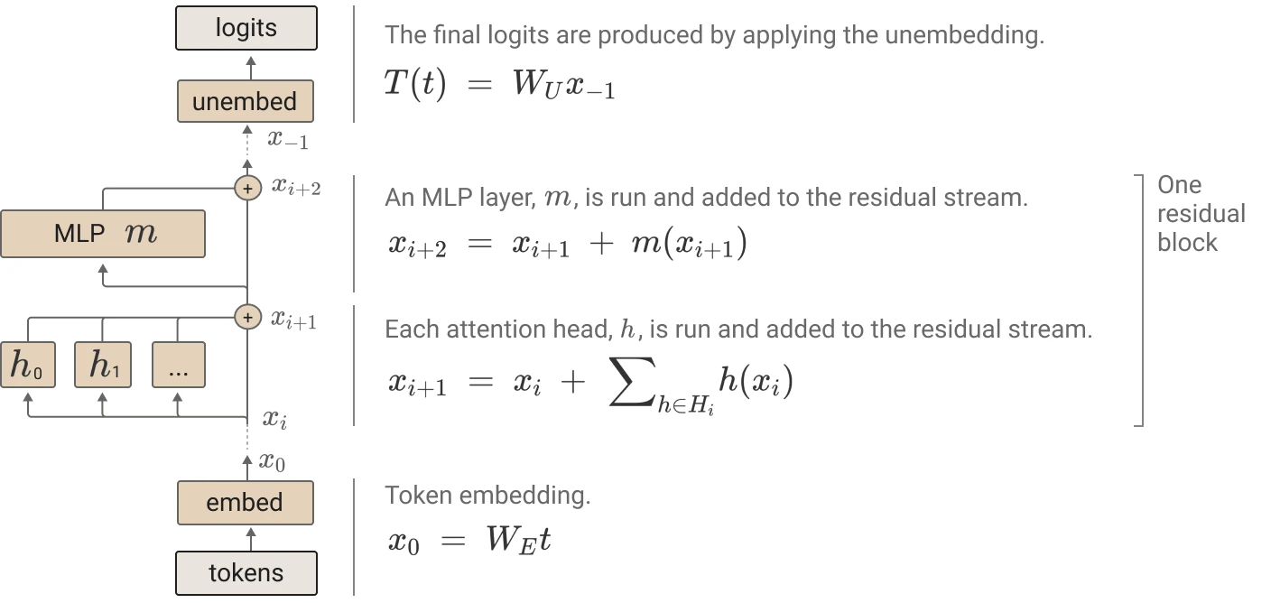
intuition: we can think of residual as highway networks, in a sense portrays linearity of the network 4
residual stream has dimension where
- : the number of tokens in context windows and
- : embedding dimension.
Attention mechanism process given residual stream as the result is added back to :
grokking
See also: writeup, code, circuit threads
A phenomena discovered by (Power et al., 2022) where small algorithmic tasks like modular addition will initially memorise training data, but after a long time ti will suddenly learn to generalise to unseen data
empirical claims
related to phase change

